Note
Click here to download the full example code
Tutorial 3: Null models for gradient significance
In this tutorial we assess the significance of correlations between the first canonical gradient and data from other modalities (curvature, cortical thickness and T1w/T2w image intensity). A normal test of the significance of the correlation cannot be used, because the spatial auto-correlation in MRI data may bias the test statistic. In this tutorial we will show three approaches for null hypothesis testing: spin permutations, Moran spectral randomization, and autocorrelation-preserving surrogates based on variogram matching.
Note
When using either approach to compare gradients to non-gradient markers, we recommend randomizing the non-gradient markers as these randomizations need not maintain the statistical independence between gradients.
Spin Permutations
Here, we use the spin permutations approach previously proposed in (Alexander-Bloch et al., 2018), which preserves the auto-correlation of the permuted feature(s) by rotating the feature data on the spherical domain. We will start by loading the conte69 surfaces for left and right hemispheres, their corresponding spheres, midline mask, and t1w/t2w intensity as well as cortical thickness data, and a template functional gradient.
import numpy as np
from brainspace.datasets import load_gradient, load_marker, load_conte69

# load the conte69 hemisphere surfaces and spheres
surf_lh, surf_rh = load_conte69()
sphere_lh, sphere_rh = load_conte69(as_sphere=True)

# Load the data
t1wt2w_lh, t1wt2w_rh = load_marker('t1wt2w')
t1wt2w = np.concatenate([t1wt2w_lh, t1wt2w_rh])

thickness_lh, thickness_rh = load_marker('thickness')
thickness = np.concatenate([thickness_lh, thickness_rh])

# Template functional gradient
embedding = load_gradient('fc', idx=0, join=True)
Let’s first generate some null data using spintest.
from brainspace.null_models import SpinPermutations
from brainspace.plotting import plot_hemispheres

# Let's create some rotations
n_rand = 1000

sp = SpinPermutations(n_rep=n_rand, random_state=0)
sp.fit(sphere_lh, points_rh=sphere_rh)

t1wt2w_rotated = np.hstack(sp.randomize(t1wt2w_lh, t1wt2w_rh))
thickness_rotated = np.hstack(sp.randomize(thickness_lh, thickness_rh))
As an illustration of the rotation, let’s plot the original t1w/t2w data
# Plot original data
plot_hemispheres(surf_lh, surf_rh, array_name=t1wt2w, size=(1200, 200), cmap='viridis',
                 nan_color=(0.5, 0.5, 0.5, 1), color_bar=True, zoom=1.65)
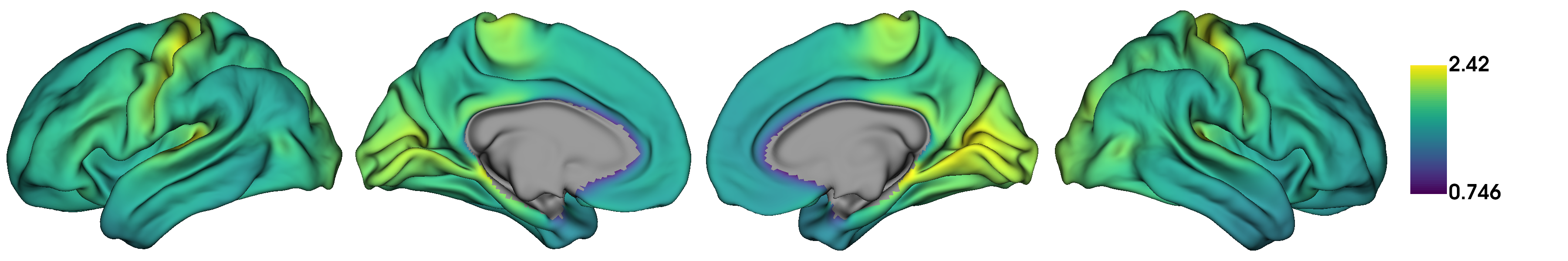
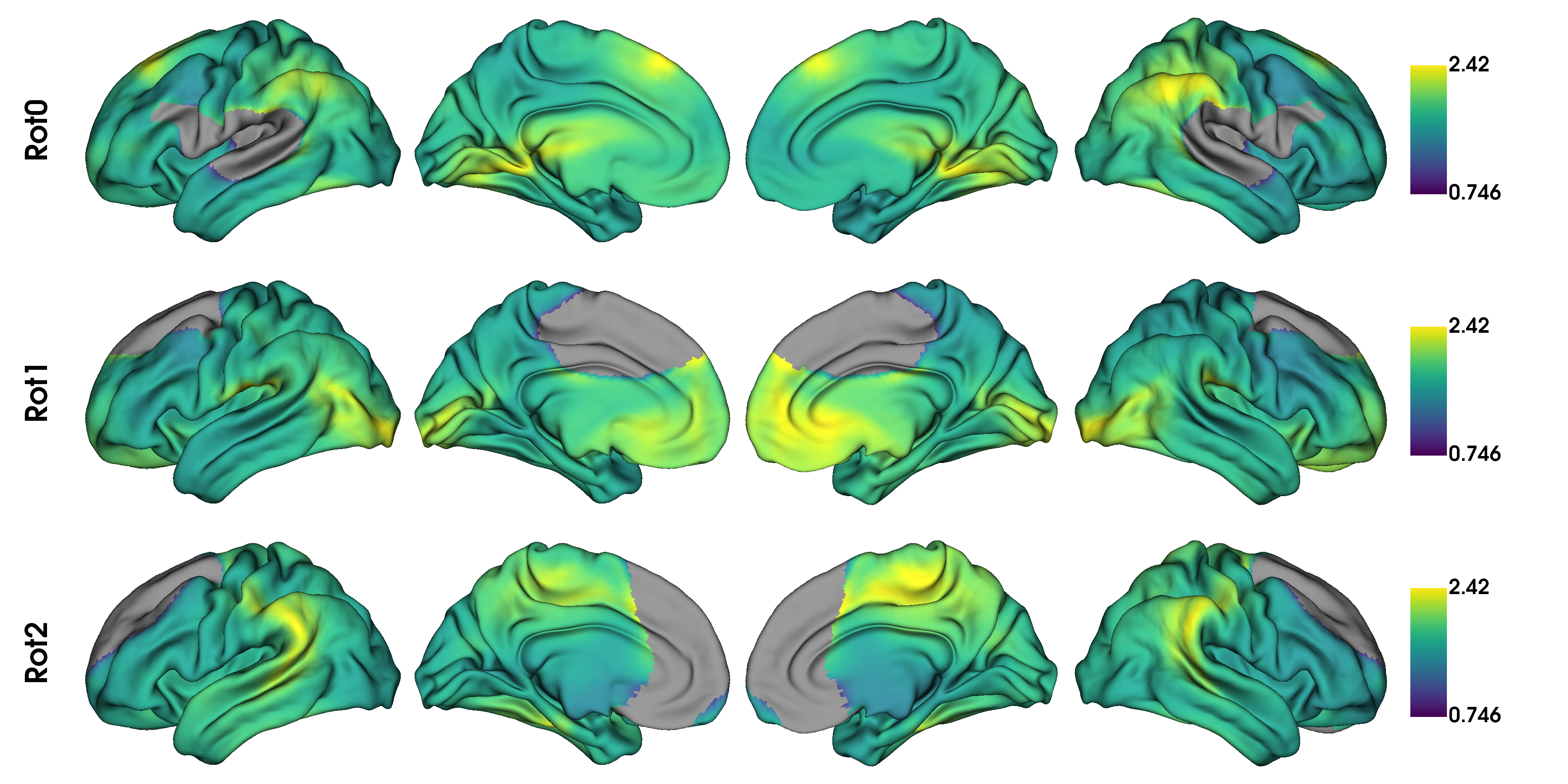
as well as a few rotated versions.
# Plot some rotations
plot_hemispheres(surf_lh, surf_rh, array_name=t1wt2w_rotated[:3], size=(1200, 600),
                 cmap='viridis', nan_color=(0.5, 0.5, 0.5, 1), color_bar=True,
                 zoom=1.55, label_text=['Rot0', 'Rot1', 'Rot2'])
Warning
With spin permutations, midline vertices (i.e,, NaNs) from both the original and rotated data are discarded. Depending on the overlap of midlines in the, statistical comparisons between them may compare different numbers of features. This can bias your test statistics. Therefore, if a large portion of the sphere is not used, we recommend using Moran spectral randomization instead.
Now we simply compute the correlations between the first gradient and the original data, as well as all rotated data.
from matplotlib import pyplot as plt
from scipy.stats import spearmanr
fig, axs = plt.subplots(1, 2, figsize=(9, 3.5))
feats = {'t1wt2w': t1wt2w, 'thickness': thickness}
rotated = {'t1wt2w': t1wt2w_rotated, 'thickness': thickness_rotated}
r_spin = np.empty(n_rand)
mask = ~np.isnan(thickness)
for k, (fn, feat) in enumerate(feats.items()):
r_obs, pv_obs = spearmanr(feat[mask], embedding[mask])
# Compute perm pval
for i, perm in enumerate(rotated[fn]):
mask_rot = mask & ~np.isnan(perm) # Remove midline
r_spin[i] = spearmanr(perm[mask_rot], embedding[mask_rot])[0]
pv_spin = np.mean(np.abs(r_spin) >= np.abs(r_obs))
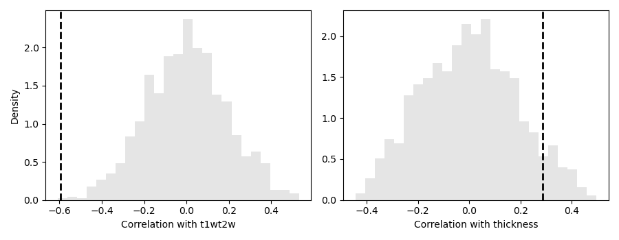
# Plot null dist
axs[k].hist(r_spin, bins=25, density=True, alpha=0.5, color=(.8, .8, .8))
axs[k].axvline(r_obs, lw=2, ls='--', color='k')
axs[k].set_xlabel(f'Correlation with {fn}')
if k == 0:
axs[k].set_ylabel('Density')
print(f'{fn.capitalize()}:\n Obs : {pv_obs:.5e}\n Spin: {pv_spin:.5e}\n')
fig.tight_layout()
plt.show()
Out:
T1wt2w:
 Obs : 0.00000e+00
 Spin: 1.00000e-03

Thickness:
 Obs : 0.00000e+00
 Spin: 1.37000e-01
It is interesting to see that both p-values increase when taking into consideration the auto-correlation present in the surfaces. Also, we can see that the correlation with thickness is no longer statistically significant after spin permutations.
Moran Spectral Randomization
Moran Spectral Randomization (MSR) computes Moran’s I, a metric for spatial auto-correlation and generates normally distributed data with similar auto-correlation. MSR relies on a weight matrix denoting the spatial proximity of features to one another. Within neuroimaging, one straightforward example of this is inverse geodesic distance i.e. distance along the cortical surface.
In this example we will show how to use MSR to assess statistical significance between cortical markers (here curvature and cortical t1wt2w intensity) and the first functional connectivity gradient. We will start by loading the left temporal lobe mask, t1w/t2w intensity as well as cortical thickness data, and a template functional gradient
from brainspace.datasets import load_mask

n_pts_lh = surf_lh.n_points
mask_tl, _ = load_mask(name='temporal')

# Keep only the temporal lobe.
embedding_tl = embedding[:n_pts_lh][mask_tl]
t1wt2w_tl = t1wt2w_lh[mask_tl]
curv_tl = load_marker('curvature')[0][mask_tl]
We will now compute the Moran eigenvectors. This can be done either by providing a weight matrix of spatial proximity between each vertex, or by providing a cortical surface. Here we’ll use a cortical surface.
from brainspace.null_models import MoranRandomization
from brainspace.mesh import mesh_elements as me

# compute spatial weight matrix
w = me.get_ring_distance(surf_lh, n_ring=1, mask=mask_tl)
w.data **= -1


msr = MoranRandomization(n_rep=n_rand, procedure='singleton', tol=1e-6,
                         random_state=0)
msr.fit(w)
Out:
MoranRandomization(n_rep=1000, random_state=0, tol=1e-06)
Using the Moran eigenvectors we can now compute the randomized data.
curv_rand = msr.randomize(curv_tl)
t1wt2w_rand = msr.randomize(t1wt2w_tl)
Now that we have the randomized data, we can compute correlations between the gradient and the real/randomised data and generate the non-parametric p-values.
fig, axs = plt.subplots(1, 2, figsize=(9, 3.5))
feats = {'t1wt2w': t1wt2w_tl, 'curvature': curv_tl}
rand = {'t1wt2w': t1wt2w_rand, 'curvature': curv_rand}
for k, (fn, data) in enumerate(rand.items()):
r_obs, pv_obs = spearmanr(feats[fn], embedding_tl, nan_policy='omit')
# Compute perm pval
r_rand = np.asarray([spearmanr(embedding_tl, d)[0] for d in data])
pv_rand = np.mean(np.abs(r_rand) >= np.abs(r_obs))
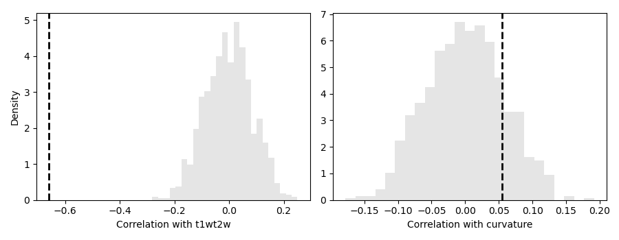
# Plot null dist
axs[k].hist(r_rand, bins=25, density=True, alpha=0.5, color=(.8, .8, .8))
axs[k].axvline(r_obs, lw=2, ls='--', color='k')
axs[k].set_xlabel(f'Correlation with {fn}')
if k == 0:
axs[k].set_ylabel('Density')
print(f'{fn.capitalize()}:\n Obs : {pv_obs:.5e}\n Moran: {pv_rand:.5e}\n')
fig.tight_layout()
plt.show()
Out:
T1wt2w:
 Obs  : 0.00000e+00
 Moran: 0.00000e+00

Curvature:
 Obs  : 6.63802e-05
 Moran: 3.50000e-01
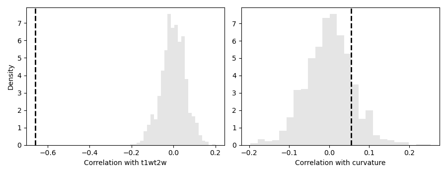
Variogram Matching
Here, we will repeat the same analysis using the variogram matching approach presented in (Burt et al., 2020), which generates novel brainmaps with similar spatial autocorrelation to the input data.
We will need a distance matrix that tells us what the spatial distance between our datapoints is. For this example, we will use geodesic distance.
from brainspace.mesh.mesh_elements import get_immediate_distance
from scipy.sparse.csgraph import dijkstra

# Compute geodesic distance
gd = get_immediate_distance(surf_lh, mask=mask_tl)
gd = dijkstra(gd, directed=False)

idx_sorted = np.argsort(gd, axis=1)
Now we’ve got everything we need to generate our surrogate datasets. By default, BrainSpace will use all available data to generate surrogate maps. However, this process is extremely computationally and memory intensive. When using this method with more than a few hundred regions, we recommend subsampling the data. This can be done using SampledSurrogateMaps instead of the SurrogateMaps.
from brainspace.null_models import SampledSurrogateMaps


n_surrogate_datasets = 1000

# Note: number samples must be greater than number neighbors
num_samples = 100
num_neighbors = 50

ssm = SampledSurrogateMaps(ns=num_samples, knn=num_neighbors, random_state=0)
ssm.fit(gd, idx_sorted)

t1wt2w_surrogates = ssm.randomize(t1wt2w_tl, n_rep=n_surrogate_datasets)
curv_surrogates = ssm.randomize(curv_tl, n_rep=n_surrogate_datasets)
Similar to the previous case, we can now plot the results:
import matplotlib.pyplot as plt
from scipy.stats import spearmanr
fig, axs = plt.subplots(1, 2, figsize=(9, 3.5))

feats = {'t1wt2w': t1wt2w_tl, 'curvature': curv_tl}
rand = {'t1wt2w': t1wt2w_surrogates, 'curvature': curv_surrogates}

for k, (fn, data) in enumerate(rand.items()):
    r_obs, pv_obs = spearmanr(feats[fn], embedding_tl, nan_policy='omit')

    # Compute perm pval
    r_rand = np.asarray([spearmanr(embedding_tl, d)[0] for d in data])
    pv_rand = np.mean(np.abs(r_rand) >= np.abs(r_obs))

    # Plot null dist
    axs[k].hist(r_rand, bins=25, density=True, alpha=0.5, color=(.8, .8, .8))
    axs[k].axvline(r_obs, lw=2, ls='--', color='k')
    axs[k].set_xlabel(f'Correlation with {fn}')
    if k == 0:
        axs[k].set_ylabel('Density')

    print(f'{fn.capitalize()}:\n Obs      : {pv_obs:.5e}\n '
          f'Variogram: {pv_rand:.5e}\n')

fig.tight_layout()
plt.show()
Out:
T1wt2w:
 Obs      : 0.00000e+00
 Variogram: 0.00000e+00

Curvature:
 Obs      : 6.63802e-05
 Variogram: 3.26000e-01
Total running time of the script: ( 3 minutes 29.601 seconds)