Tutorial 2: Customizing and aligning gradients

In this tutorial you’ll learn about the methods available within the GradientMaps class. The flexible usage of this class allows for the customization of gradient computation with different kernels and dimensionality reductions, as well as aligning gradients from different datasets. This tutorial will only show you how to apply these techniques.

Customizing gradient computation

As before, we’ll start by loading the sample data.

from brainspace.datasets import load_group_fc, load_parcellation, load_conte69

# First load mean connectivity matrix and Schaefer parcellation
conn_matrix = load_group_fc('schaefer', scale=400)
labeling = load_parcellation('schaefer', scale=400, join=True)

mask = labeling != 0

# and load the conte69 hemisphere surfaces
surf_lh, surf_rh = load_conte69()

The GradientMaps object allows for many different kernels and dimensionality reduction techniques. Let’s have a look at three different kernels.

import numpy as np

from brainspace.gradient import GradientMaps
from brainspace.plotting import plot_hemispheres
from brainspace.utils.parcellation import map_to_labels

kernels = ['pearson', 'spearman', 'normalized_angle']

gradients_kernel = [None] * len(kernels)
for i, k in enumerate(kernels):
    gm = GradientMaps(kernel=k, approach='dm', random_state=0)
    gm.fit(conn_matrix)

    gradients_kernel[i] = map_to_labels(gm.gradients_[:, i], labeling, mask=mask,
                                        fill=np.nan)


label_text = ['Pearson', 'Spearman', 'Normalized\nAngle']
plot_hemispheres(surf_lh, surf_rh, array_name=gradients_kernel, size=(1200, 600),
                 cmap='viridis_r', color_bar=True, label_text=label_text, zoom=1.45)

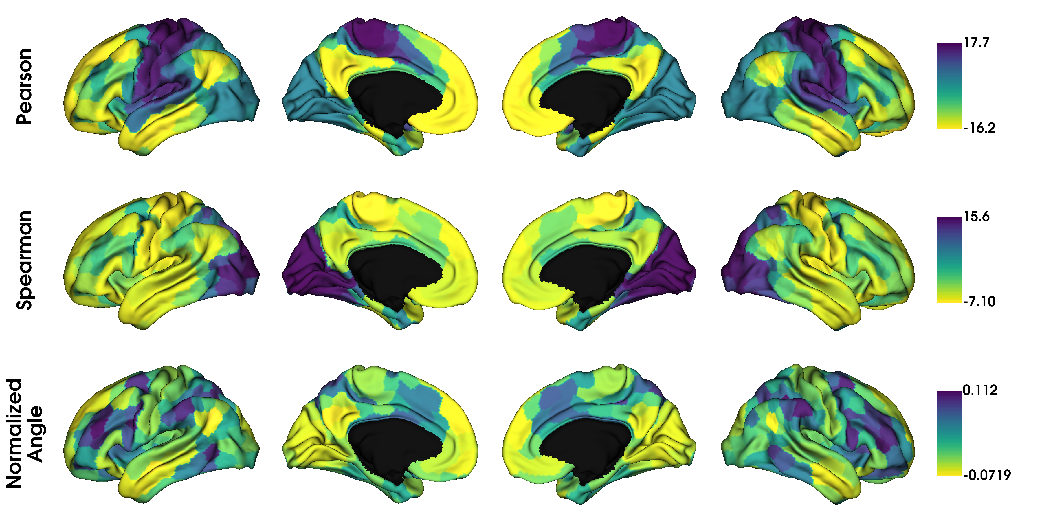
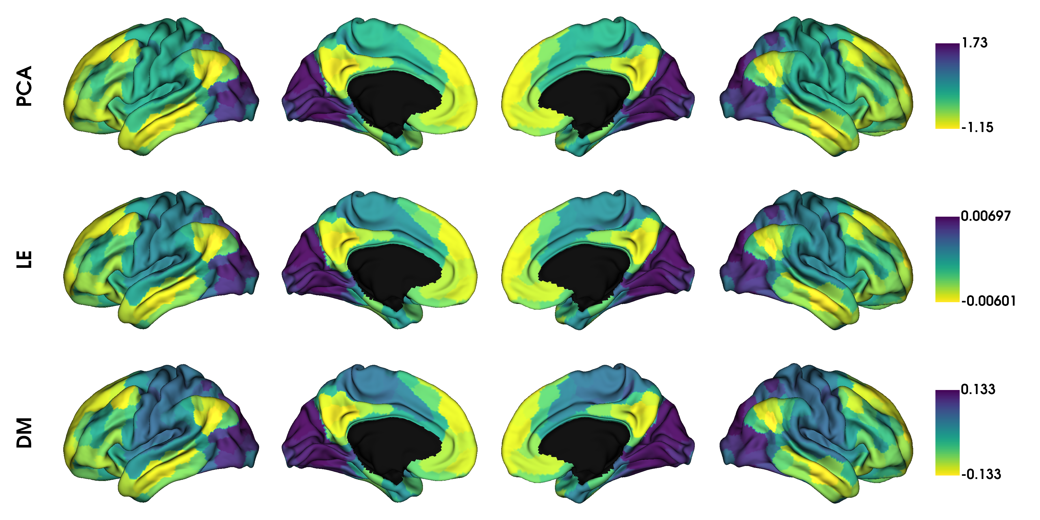
It seems the gradients provided by these kernels are quite similar although their scaling is quite different. Do note that the gradients are in arbitrary units, so the smaller/larger axes across kernels do not imply anything. Similar to using different kernels, we can also use different dimensionality reduction techniques.

# PCA, Laplacian eigenmaps and diffusion mapping
embeddings = ['pca', 'le', 'dm']

gradients_embedding = [None] * len(embeddings)
for i, emb in enumerate(embeddings):
    gm = GradientMaps(kernel='normalized_angle', approach=emb, random_state=0)
    gm.fit(conn_matrix)

    gradients_embedding[i] = map_to_labels(gm.gradients_[:, 0], labeling, mask=mask,
                                           fill=np.nan)


label_text = ['PCA', 'LE', 'DM']
plot_hemispheres(surf_lh, surf_rh, array_name=gradients_embedding, size=(1200, 600),
                 cmap='viridis_r', color_bar=True, label_text=label_text, zoom=1.45)

Gradient alignment

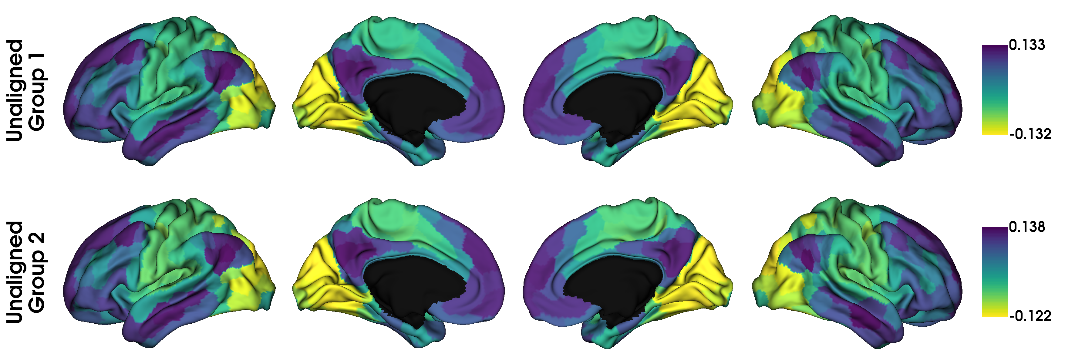
A more principled way of increasing comparability across gradients are alignment techniques. BrainSpace provides two alignment techniques: Procrustes analysis, and joint alignment. For this example we will load functional connectivity data of a second subject group and align it with the first group.

conn_matrix2 = load_group_fc('schaefer', scale=400, group='holdout')
gp = GradientMaps(kernel='normalized_angle', alignment='procrustes')
gj = GradientMaps(kernel='normalized_angle', alignment='joint')

gp.fit([conn_matrix, conn_matrix2])
gj.fit([conn_matrix, conn_matrix2])

Out:

GradientMaps(alignment='joint', kernel='normalized_angle')

Here, gp contains the Procrustes aligned data and gj contains the joint aligned data. Let’s plot them, but in separate figures to keep things organized.

# First gradient from original and holdout data, without alignment
gradients_unaligned = [None] * 2
for i in range(2):
    gradients_unaligned[i] = map_to_labels(gp.gradients_[i][:, 0], labeling,
                                           mask=mask, fill=np.nan)

label_text = ['Unaligned\nGroup 1', 'Unaligned\nGroup 2']
plot_hemispheres(surf_lh, surf_rh, array_name=gradients_unaligned, size=(1200, 400),
                 cmap='viridis_r', color_bar=True, label_text=label_text, zoom=1.5)

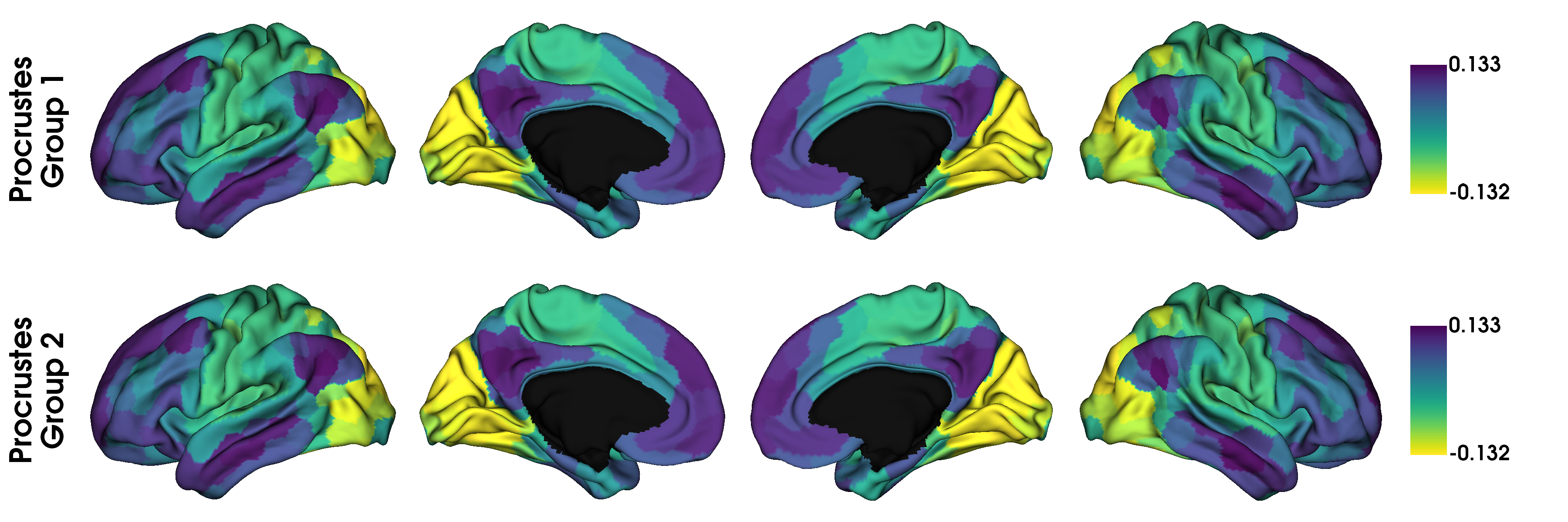
# With procrustes alignment
gradients_procrustes = [None] * 2
for i in range(2):
    gradients_procrustes[i] = map_to_labels(gp.aligned_[i][:, 0], labeling, mask=mask,
                                            fill=np.nan)

label_text = ['Procrustes\nGroup 1', 'Procrustes\nGroup 2']
plot_hemispheres(surf_lh, surf_rh, array_name=gradients_procrustes, size=(1200, 400),
                 cmap='viridis_r', color_bar=True, label_text=label_text, zoom=1.5)

# With joint alignment
gradients_joint = [None] * 2
for i in range(2):
    gradients_joint[i] = map_to_labels(gj.aligned_[i][:, 0], labeling, mask=mask,
                                       fill=np.nan)

label_text = ['Joint\nGroup 1', 'Joint\nGroup 2']
plot_hemispheres(surf_lh, surf_rh, array_name=gradients_joint, size=(1200, 400),
                 cmap='viridis_r', color_bar=True, label_text=label_text, zoom=1.5)

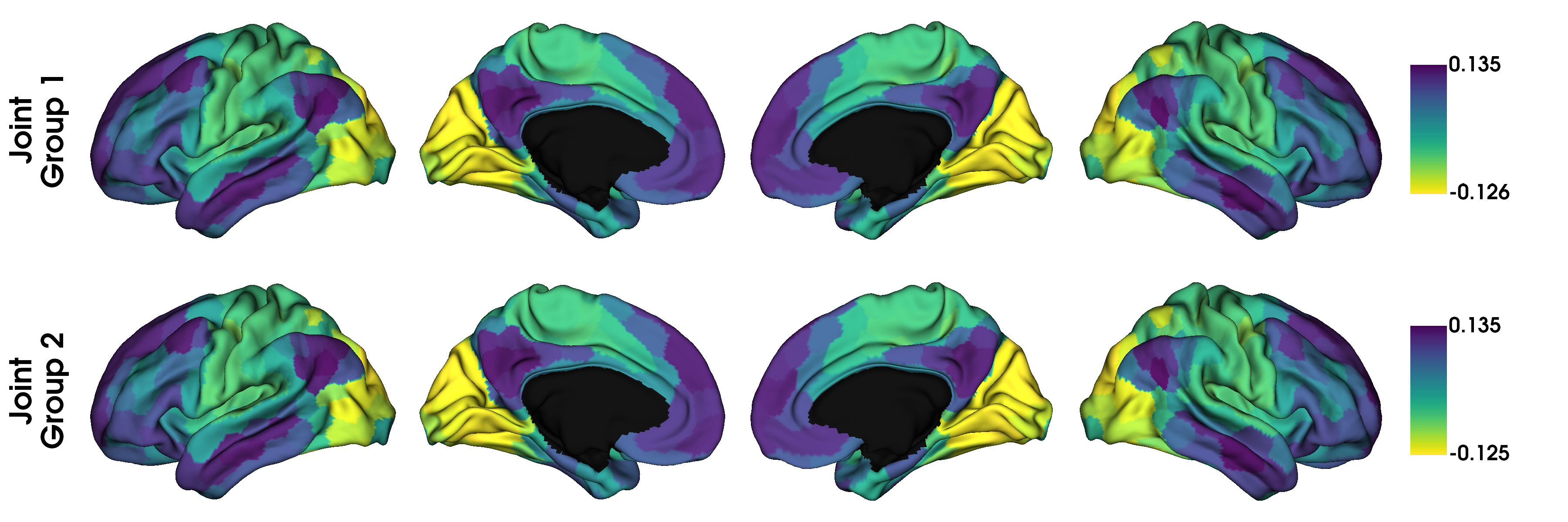
Although in this example, we don’t see any big differences, if the input data was less similar, alignments may also resolve changes in the order of the gradients. However, you should always inspect the output of an alignment; if the input data are sufficiently dissimilar then the alignment may produce odd results.

In some instances, you may want to align gradients to an out-of-sample gradient, for example when aligning individuals to a hold-out group gradient. When performing a Procrustes alignemnt, a ‘reference’ can be specified. The first alignment iteration will then be to the reference. For purposes of this example, we will use the gradient of the hold-out group as the reference.

gref = GradientMaps(kernel='normalized_angle', approach='le')
gref.fit(conn_matrix2)

galign = GradientMaps(kernel='normalized_angle', approach='le', alignment='procrustes')
galign.fit(conn_matrix, reference=gref.gradients_)

Out:

GradientMaps(alignment='procrustes', approach='le', kernel='normalized_angle')

The gradients in galign.aligned_ are now aligned to the reference gradients.

Gradient fusion

We can also fuse data across multiple modalities and build mutli-modal gradients. In this case we only look at one set of output gradients, rather than one per modality.

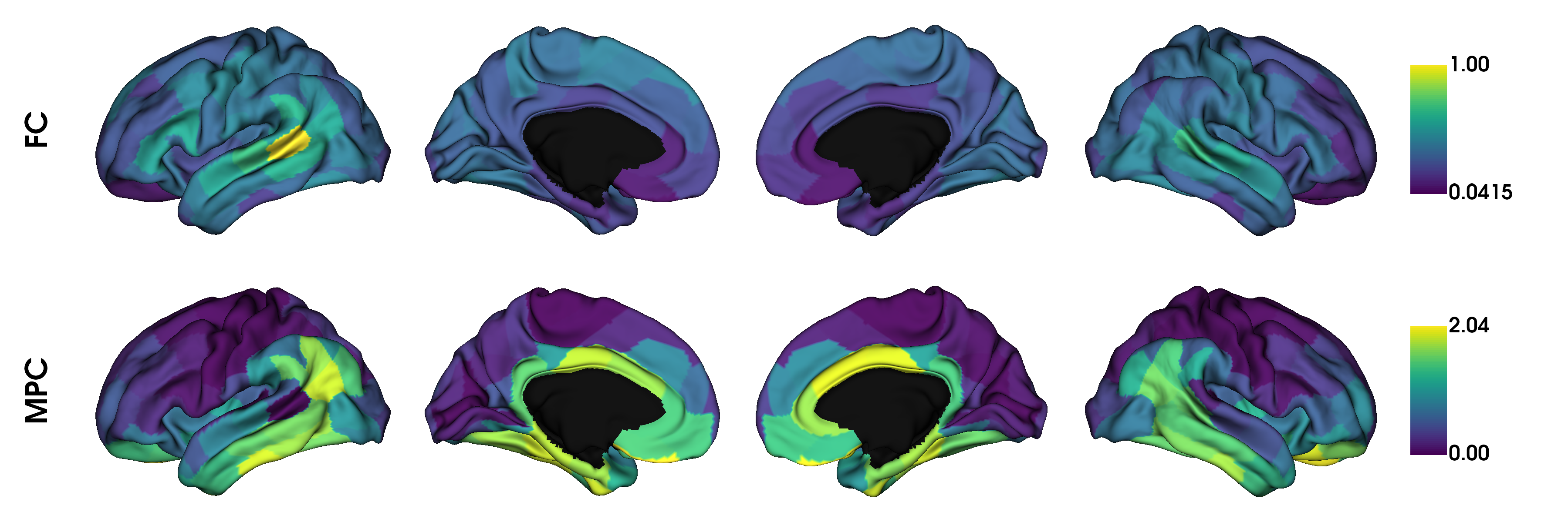
First, let’s load the example data of microstructural profile covariance (Paquola et al., 2019) and functional connectivity.

from brainspace.datasets import load_group_mpc

# First load mean connectivity matrix and parcellation
fc = load_group_fc('vosdewael', scale=200)
mpc = load_group_mpc('vosdewael', scale=200)

labeling = load_parcellation('vosdewael', scale=200, join=True)
mask = labeling != 0

seeds = [None] * 2
seeds[0] = map_to_labels(fc[0], labeling, mask=mask, fill=np.nan)
seeds[1] = map_to_labels(mpc[0], labeling, mask=mask, fill=np.nan)

# visualise the features from a seed region (seed 0)
plot_hemispheres(surf_lh, surf_rh, array_name=seeds, label_text=['FC', 'MPC'],
                 size=(1200, 400), color_bar=True, cmap='viridis', zoom=1.45)

In order to fuse the matrices, we simply pass the matrices to the fusion command which will rescale and horizontally concatenate the matrices.

# Negative numbers are not allowed in fusion.
fc[fc < 0] = 0


def fusion(*args):
    from scipy.stats import rankdata
    from sklearn.preprocessing import minmax_scale

    max_rk = [None] * len(args)
    masks = [None] * len(args)
    for j, a in enumerate(args):
        m = masks[j] = a != 0
        a[m] = rankdata(a[m])
        max_rk[j] = a[m].max()

    max_rk = min(max_rk)
    for j, a in enumerate(args):
        m = masks[j]
        a[m] = minmax_scale(a[m], feature_range=(1, max_rk))

    return np.hstack(args)


# fuse the matrices
fused_matrix = fusion(fc, mpc)

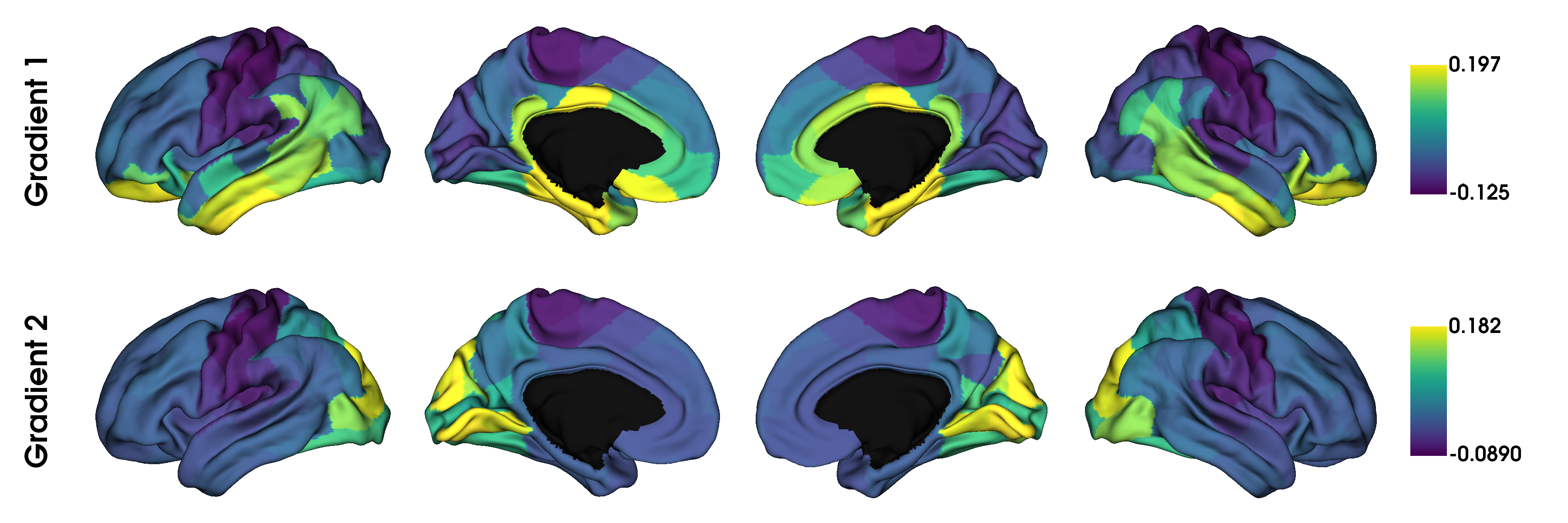
We then use this output in the fit function. This will convert the long horizontal array into a square affinity matrix, and then perform embedding.

gm = GradientMaps(n_components=2, kernel='normalized_angle')
gm.fit(fused_matrix)


gradients_fused = [None] * 2
for i in range(2):
    gradients_fused[i] = map_to_labels(gm.gradients_[:, i], labeling, mask=mask,
                                       fill=np.nan)

plot_hemispheres(surf_lh, surf_rh, array_name=gradients_fused,
                 label_text=['Gradient 1', 'Gradient 2'], size=(1200, 400),
                 color_bar=True, cmap='viridis', zoom=1.45)

Note

The mpc matrix presented here matches the subject cohort of (Paquola et al., 2019). Other matrices in this package match the subject groups used by (Vos de Wael et al., 2018). We make direct comparisons in our tutorial for didactic purposes only.

That concludes the second tutorial. In the third tutorial we will consider null hypothesis testing of comparisons between gradients and other markers.