Tutorial 0: Preparing your data for gradient analysis

In this example, we will introduce how to preprocess raw MRI data and how to prepare it for subsequent gradient analysis in the next tutorials.

Requirements

For this tutorial, you will need to install the Python package nilearn version 0.9.0 or above. You can do it using pip:

pip install "nilearn>=0.9.0"

Preprocessing

Begin with an MRI dataset that is organized in BIDS format. We recommend preprocessing your data using fmriprep, as described below, but any preprocessing pipeline will work.

Following is example code to run fmriprep using docker from the command line:

docker run -ti --rm \
  -v <local_BIDS_data_dir>:/data:ro \
  -v <local_output_dir>:/out poldracklab/fmriprep:latest \
  --output-spaces fsaverage5 \
  --fs-license-file license.txt \
  /data /out participant

Note

For this tutorial, it is crucial to output the data onto a cortical surface template space.

Import the dataset as timeseries

The timeseries should be a numpy array with the dimensions: nodes x timepoints

Following is an example for reading in data:

import nibabel as nib
import numpy as np

filename = 'filename.{}.mgz' # where {} will be replaced with 'lh' and 'rh'
timeseries = [None] * 2
for i, h in enumerate(['lh', 'rh']):
    timeseries[i] = nib.load(filename.format(h)).get_fdata().squeeze()
timeseries = np.vstack(timeseries)

As a working example, simply fetch timeseries:

from brainspace.datasets import fetch_timeseries_preprocessing
timeseries = fetch_timeseries_preprocessing()

Confound regression

To remove confound regressors from the output of the fmriprep pipeline, first extract the confound columns. For example:

from nilearn.interfaces.fmriprep import load_confounds_strategy
confounds_out = load_confounds_strategy("path/to/fmriprep/output/sub-<subject>_task-<task>_space-<space>_desc-preproc_bold.nii.gz",
                                        denoise_strategy='simple')

As a working example, simply read in confounds

from brainspace.datasets import load_confounds_preprocessing
confounds_out = load_confounds_preprocessing()

Do the confound regression

from nilearn import signal
clean_ts = signal.clean(timeseries.T, confounds=confounds_out).T

And extract the cleaned timeseries onto a set of labels

import numpy as np
from nilearn import datasets
from brainspace.utils.parcellation import reduce_by_labels

# Fetch surface atlas
atlas = datasets.fetch_atlas_surf_destrieux()

# Remove non-cortex regions
regions = atlas['labels'].copy()
masked_regions = [b'Medial_wall', b'Unknown']
masked_labels = [regions.index(r) for r in masked_regions]
for r in masked_regions:
    regions.remove(r)

# Build Destrieux parcellation and mask
labeling = np.concatenate([atlas['map_left'], atlas['map_right']])
mask = ~np.isin(labeling, masked_labels)

# Distinct labels for left and right hemispheres
lab_lh = atlas['map_left']
labeling[lab_lh.size:] += lab_lh.max() + 1

# extract mean timeseries for each label
seed_ts = reduce_by_labels(clean_ts[mask], labeling[mask], axis=1, red_op='mean')

Out:

/home/oualid/Apps/anaconda3/envs/py3/lib/python3.7/site-packages/nilearn/datasets/__init__.py:89: FutureWarning: Fetchers from the nilearn.datasets module will be updated in version 0.9 to return python strings instead of bytes and Pandas dataframes instead of Numpy arrays.
  "Numpy arrays.", FutureWarning)

Dataset created in /home/oualid/nilearn_data/destrieux_surface

Downloading data from https://www.nitrc.org/frs/download.php/9343/lh.aparc.a2009s.annot ...
 ...done. (0 seconds, 0 min)
Downloading data from https://www.nitrc.org/frs/download.php/9342/rh.aparc.a2009s.annot ...
 ...done. (0 seconds, 0 min)

Calculate functional connectivity matrix

The following example uses nilearn:

from nilearn.connectome import ConnectivityMeasure

correlation_measure = ConnectivityMeasure(kind='correlation')
correlation_matrix = correlation_measure.fit_transform([seed_ts.T])[0]

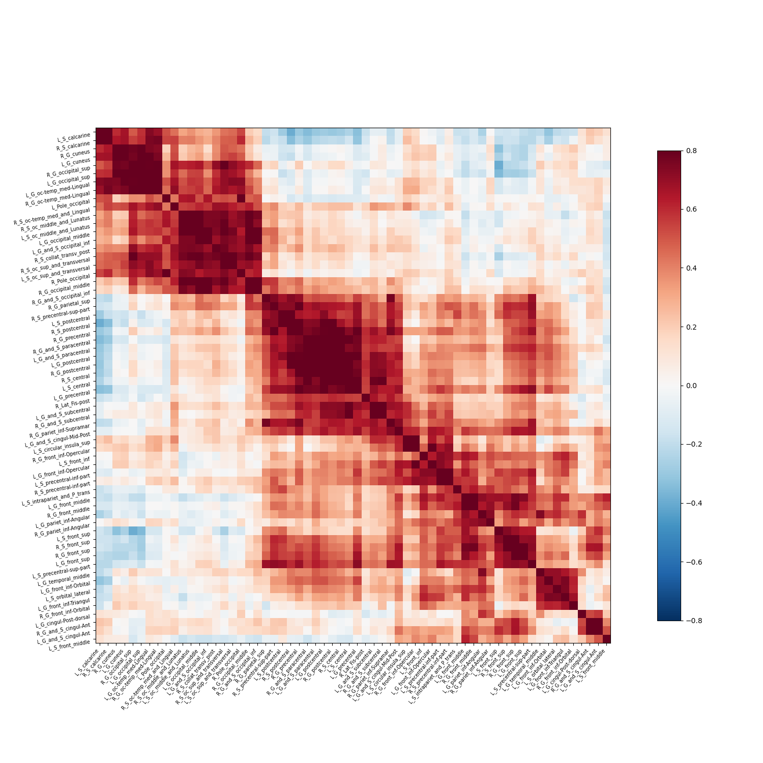
Plot the correlation matrix:

from nilearn import plotting

# Reduce matrix size, only for visualization purposes
mat_mask = np.where(np.std(correlation_matrix, axis=1) > 0.2)[0]
c = correlation_matrix[mat_mask][:, mat_mask]

# Create corresponding region names
regions_list = ['%s_%s' % (h, r.decode()) for h in ['L', 'R'] for r in regions]
masked_regions = [regions_list[i] for i in mat_mask]


corr_plot = plotting.plot_matrix(c, figure=(15, 15), labels=masked_regions,
                                 vmax=0.8, vmin=-0.8, reorder=True)

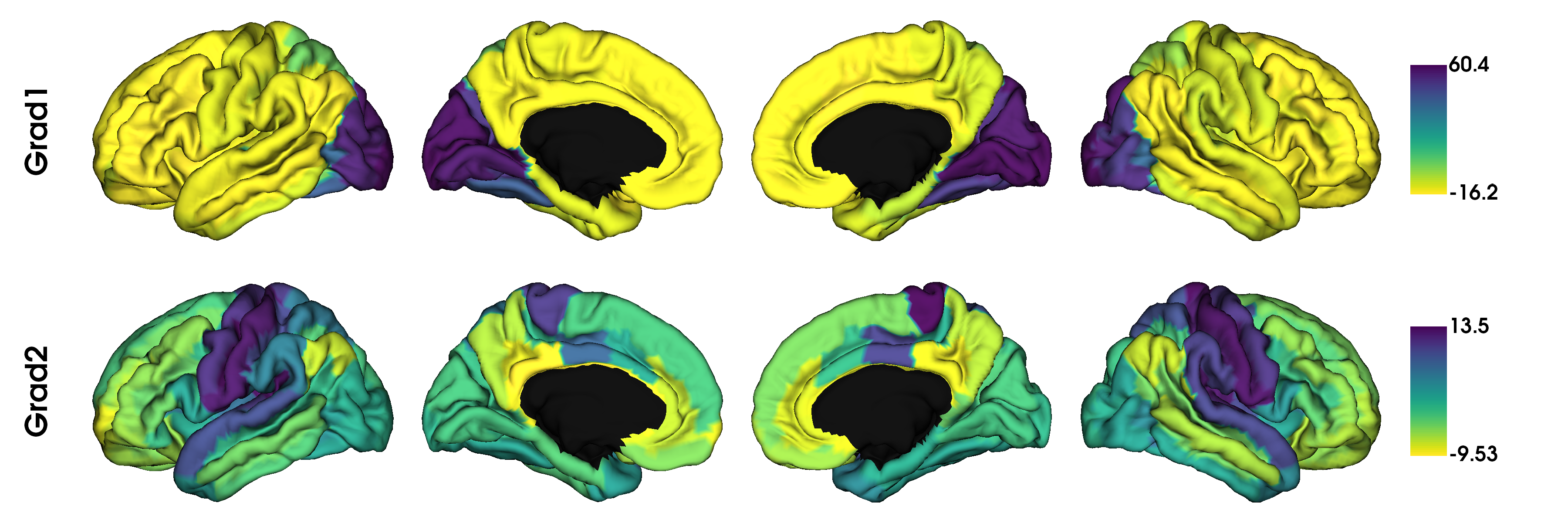
Run gradient analysis and visualize

Run gradient analysis

from brainspace.gradient import GradientMaps

gm = GradientMaps(n_components=2, random_state=0)
gm.fit(correlation_matrix)

Out:

GradientMaps(n_components=2, random_state=0)

Visualize results

from brainspace.datasets import load_fsa5
from brainspace.plotting import plot_hemispheres
from brainspace.utils.parcellation import map_to_labels

# Map gradients to original parcels
grad = [None] * 2
for i, g in enumerate(gm.gradients_.T):
    grad[i] = map_to_labels(g, labeling, mask=mask, fill=np.nan)


# Load fsaverage5 surfaces
surf_lh, surf_rh = load_fsa5()

plot_hemispheres(surf_lh, surf_rh, array_name=grad, size=(1200, 400), cmap='viridis_r',
                 color_bar=True, label_text=['Grad1', 'Grad2'], zoom=1.5)

This concludes the setup tutorial. The following tutorials can be run using either the output generated here or the example data.