Tutorial 1: Building your first gradient

In this example, we will derive a gradient and do some basic inspections to determine which gradients may be of interest and what the multidimensional organization of the gradients looks like.

We’ll first start by loading some sample data. Note that we’re using parcellated data for computational efficiency.

from brainspace.datasets import load_group_fc, load_parcellation, load_conte69

# First load mean connectivity matrix and Schaefer parcellation
conn_matrix = load_group_fc('schaefer', scale=400)
labeling = load_parcellation('schaefer', scale=400, join=True)

# and load the conte69 surfaces
surf_lh, surf_rh = load_conte69()

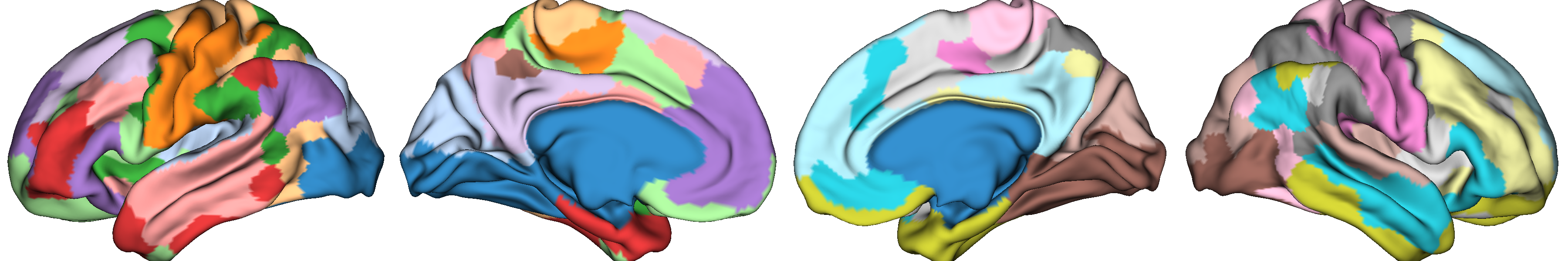
Let’s first look at the parcellation scheme we’re using.

from brainspace.plotting import plot_hemispheres

plot_hemispheres(surf_lh, surf_rh, array_name=labeling, size=(1200, 200),
                 cmap='tab20', zoom=1.85)

and let’s construct our gradients.

from brainspace.gradient import GradientMaps

# Ask for 10 gradients (default)
gm = GradientMaps(n_components=10, random_state=0)
gm.fit(conn_matrix)

Out:

GradientMaps(random_state=0)

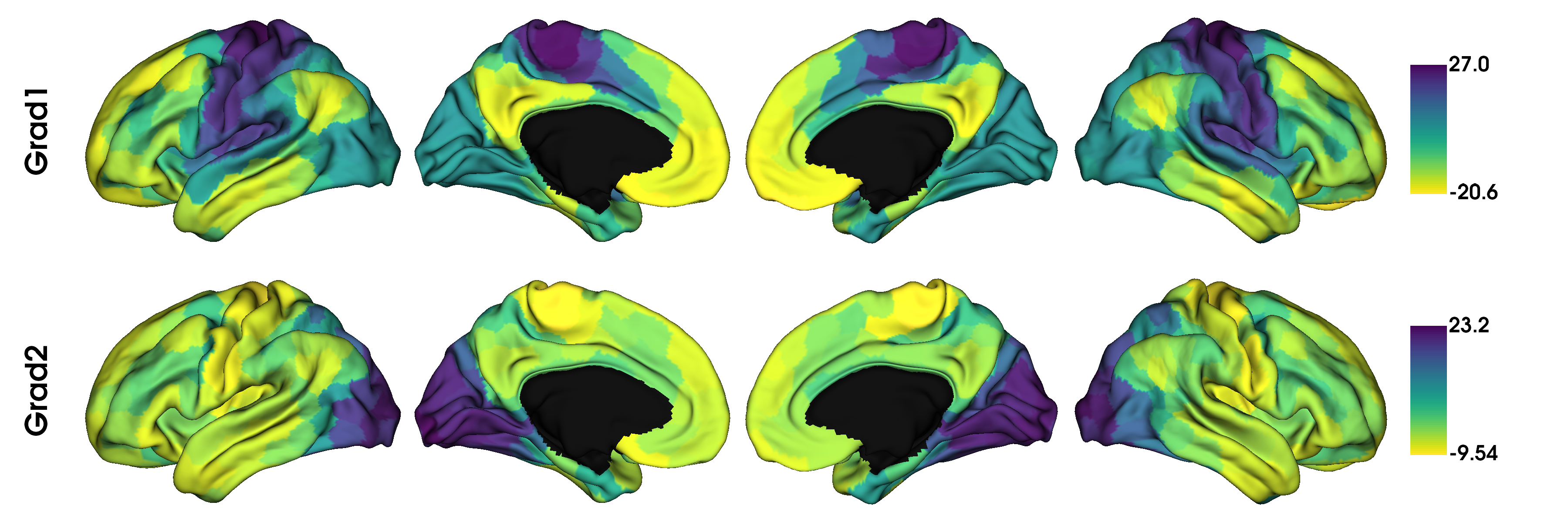
Note that the default parameters are diffusion embedding approach, 10 components, and no kernel (use raw data). Once you have your gradients, a good first step is to simply inspect what they look like. Let’s have a look at the first two gradients.

import numpy as np

from brainspace.utils.parcellation import map_to_labels

mask = labeling != 0

grad = [None] * 2
for i in range(2):
    # map the gradient to the parcels
    grad[i] = map_to_labels(gm.gradients_[:, i], labeling, mask=mask, fill=np.nan)

plot_hemispheres(surf_lh, surf_rh, array_name=grad, size=(1200, 400), cmap='viridis_r',
                 color_bar=True, label_text=['Grad1', 'Grad2'], zoom=1.55)

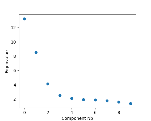
But which gradients should you keep for your analysis? In some cases you may have an a priori interest in some previously defined set of gradients. When you do not have a pre-defined set, you can instead look at the lambdas (eigenvalues) of each component in a scree plot. Higher eigenvalues (or lower in Laplacian eigenmaps) are more important, so one can choose a cut-off based on a scree plot.

import matplotlib.pyplot as plt

fig, ax = plt.subplots(1, figsize=(5, 4))
ax.scatter(range(gm.lambdas_.size), gm.lambdas_)
ax.set_xlabel('Component Nb')
ax.set_ylabel('Eigenvalue')

plt.show()

This concludes the first tutorial. In the next tutorial we will have a look at how to customize the methods of gradient estimation, as well as gradient alignments.