Tutorial 2: Customizing and aligning gradients

In this tutorial you’ll learn about the methods available within the GradientMaps class. The flexible usage of this class allows for the customization of gradient computation with different kernels and dimensionality reductions, as well as aligning gradients from different datasets. This tutorial will only show you how to apply these techniques, for in-depth descriptions we recommend you read the main manuscript.

Customizing Gradient Computation

As before, we’ll start by loading the sample data.

% First load mean connectivity matrix and Schaefer parcellation
conn_matrix = load_group_fc('schaefer',400);
labeling = load_parcellation('schaefer',400);

% The loader functions output data in a struct array for when you
% load multiple parcellations. Let's just bring them to numeric arrays.
conn_matrix = conn_matrix.schaefer_400;
labeling = labeling.schaefer_400;

% and load the conte69 hemisphere surfaces
[surf_lh, surf_rh] = load_conte69();

The GradientMaps object allows for many different kernels and dimensionality reduction techniques (for a full list see GradientMaps). Let’s have a look at three different kernels.

kernels = {'pearson', ...
           'spearman', ...
           'normalizedAngle'}; % Case-insensitive
for ii = 1:numel(kernels)
    gm_k{ii} = GradientMaps('kernel',kernels{ii},'approach','dm');
    gm_k{ii} = gm_k{ii}.fit(conn_matrix);
end

label_text = {'Pearson','Spearman',{'Normalized','Angle'}};
plot_hemispheres([gm_k{1}.gradients{1}(:,1), ...
    gm_k{2}.gradients{1}(:,1), ...
    gm_k{3}.gradients{1}(:,1)], ...
    {surf_lh,surf_rh}, ...
    'parcellation', labeling, ...
    'labeltext',label_text);

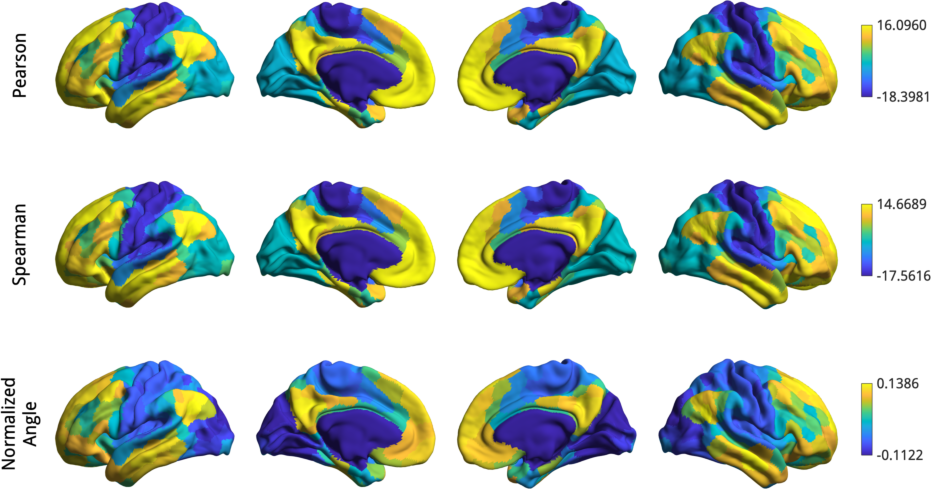
It seems the gradients provided by these kernels are quite similar although their scaling is quite different. Do note that the gradients are in arbitrary units, so the smaller/larger axes across kernels do not imply anything. Similar to using different kernels, we can also use different dimensionality reduction techniques.

% Compute gradients for every approach.
embeddings = {'principalComponentAnalysis', ...
              'laplacianEigenmap', ...
              'diffusionEmbedding'}; % case-insensitve
for ii = 1:numel(embeddings)
    gm_m{ii} = GradientMaps('kernel','na','approach',embeddings{ii});
    gm_m{ii} = gm_m{ii}.fit(conn_matrix);
end

% Plot all to one figure.
label_text = {{'Principal','Component Analysis'}, ...
    {'Laplacian','Eigenmap'}, {'Diffusion','Map Embedding'}};
plot_hemispheres([gm_m{1}.gradients{1}(:,1), ...
    gm_m{2}.gradients{1}(:,1), ...
    gm_m{3}.gradients{1}(:,1)], ...
    {surf_lh,surf_rh}, ...
    'parcellation', labeling, ...
    'labeltext', label_text);

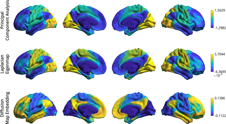
Here we do see some substantial differences: PCA appears to find a slightly different axis, with the somatomotor in the middle between default mode and visual, whereas LE and DM both find the canonical first gradient but their signs are flipped! Fortunately, the sign of gradients is arbitrary, so we could simply multiply either the LM and DM gradient by -1 to make them more comparable.

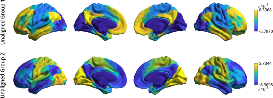
Gradient Alignment

A more principled way of increasing comparability across gradients are alignment techniques. BrainSpace provides two alignment techniques: Procrustes analysis, and joint alignment. For this example we will load functional connectivity data of a second subject group and align it with the first group using a normalized angle kernel and laplacian eigenmap approach.

conn_matrix2 = load_group_fc('schaefer',400,'holdout');
conn_matrix2 = conn_matrix2.schaefer_400;
Gp = GradientMaps('kernel','na','approach','le','alignment','pa');
Gj = GradientMaps('kernel','na','approach','le','alignment','ja');

Gp = Gp.fit({conn_matrix2,conn_matrix});
Gj = Gj.fit({conn_matrix2,conn_matrix});

Here, Gp contains the Procrustes aligned data and Gj contains the joint aligned data. Let’s plot them, but in separate figures to keep things organized. Note that the gradients in the first element of the gradients/aligned property correspond to the first data matrix provided in fit() and the gradients in the second element correspond to the second data matrix.

plot_hemispheres([Gp.gradients{1}(:,1),Gp.gradients{2}(:,1)], ...
    {surf_lh,surf_rh}, 'parcellation', labeling, ...
    'labeltext',{'Unaligned Group 1','Unaligned Group 2'});

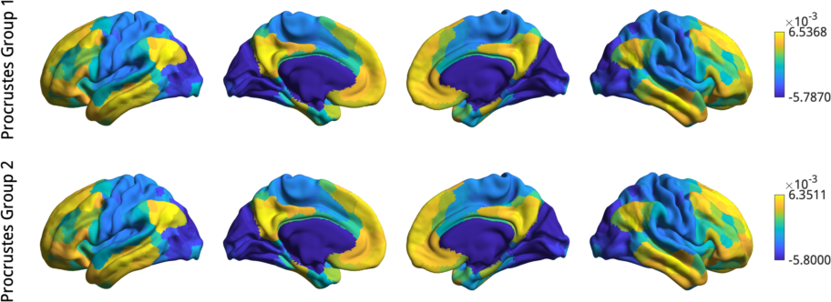
plot_hemispheres([Gp.aligned{1}(:,1),Gp.aligned{2}(:,1)], ...
    {surf_lh,surf_rh},'parcellation',labeling, ...
    'labeltext',{'Procrustes Group 1','Procrustes Group 2'});

plot_hemispheres([Gj.aligned{1}(:,1),Gj.aligned{2}(:,1)], ...
    {surf_lh,surf_rh},'parcellation',labeling, ...
    'labeltext',{'Joint Group 1','Joint Group 2'});

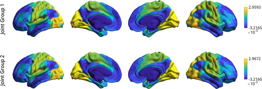
Before gradient alignment, the first gradient is reversed, but both alignments resolve this issue. If the input data was less similar, alignments may also resolve changes in the order of the gradients. However, you should always inspect the output of an alignment; if the input data are sufficiently dissimilar then the alignment may produce odd results.

In some instances, you may want to align gradients to an out-of-sample gradient, for example when aligning individuals to a hold-out group gradient. When performing a Procrustes alignemnt, a ‘reference’ can be specified. The first alignment iteration will then be to the reference. For purposes of this example, we will use the gradient of the hold-out group as the reference.

Gref = GradientMaps('kernel','na','approach','le');
Gref = Gref.fit(conn_matrix2);

Galign = GradientMaps('kernel','na','approach','le','alignment','pa');
Galign = Galign.fit(conn_matrix,'reference',Gref.gradients{1});

The gradients in Galign.aligned are now aligned to the reference gradients.

Gradient Fusion

We can also fuse data across multiple modalities and build mutli-modal gradients as was done by (Paquola et al., 2019). In this case we only look at one set of output gradients, rather than one per modality.

First, let’s load the example data of microstructural profile covariance and functional connectivity.

% First load mean connectivity matrix and parcellation
mpc = load_group_mpc('vosdewael',200);
fc = load_group_fc('vosdewael',200);
labeling = load_parcellation('vosdewael',200);

% The loader functions output data in a struct array for when you
% load multiple parcellations. Let's just bring them to numeric arrays.
mpc = mpc.vosdewael_200;
fc = fc.vosdewael_200;
labeling = labeling.vosdewael_200;

% and load the conte69 hemisphere surfaces
[surf_lh, surf_rh] = load_conte69();

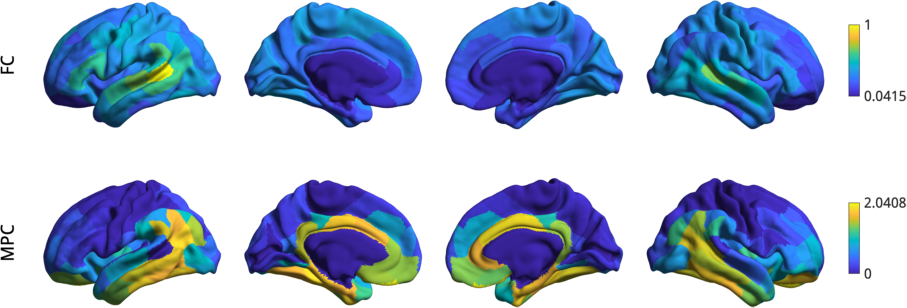
% visualise the features from a seed region
h = plot_hemispheres([fc(:,1),mpc(:,1)], ...
            {surf_lh,surf_rh}, ...
             'parcellation', labeling, ...
             'labeltext',{'FC','MPC'});

In order to fuse the matrices, we simply pass the matrices to the fusion command which will rescale and horizontally concatenate the matrices. To do this, you will need the fusion function, which is not included with the BrainSpace package.

function fused_matrix = fusion(M)
% FUSION   Fuses matrices from multiple modalities for deep embedding.
%
%   fused_matrix = fusion(M) rank orders the input
%   matrices and scales them to the maximum of the sparsest matrix.
%   M must be a cell array of matrices with the same dimensionality.

% Check the input for nans, infs, and negatives.
if any(cellfun(@(x) any(x(:)<0) || any(isnan(x(:))) || any(isinf(x(:))), M))
error('Negative numbers, nans, and infs are not allowed in the input matrices.');
end

% Check matrix sizes
sz = cellfun(@size,M,'Uniform',false);
if any(cellfun(@numel,sz) > 2)
error('Input matrices may not have more than two dimensions.')
end
if ~all(cellfun(@(x)all(x==sz{1}),sz))
error('Input matrices must have equal dimensions.')
end

% Reshape data to be a vector per input matrix
vectorized = cellfun(@(x)x(:),M,'Uniform',false);
data_matrix = cat(2,vectorized{:});
data_matrix(data_matrix==0) = nan;

% Get rank order and scale to 1 through the maximum of the smallest rank
ranking = tiedrank(data_matrix);
max_val = min(max(ranking));
rank_scaled = rescale(ranking,1,max_val,'InputMin',min(ranking),'InputMax',max(ranking));

% Reshape to output format and remove nans.
fused_matrix = reshape(rank_scaled, size(M{1},1), []);
fused_matrix(isnan(fused_matrix)) = 0;
end

With this function in your path, you can now run the following.

% Negative numbers are not allowed in fusion.
fc(fc<0) = 0;

% fuse the matrices
fused_matrix = fusion({fc,mpc});

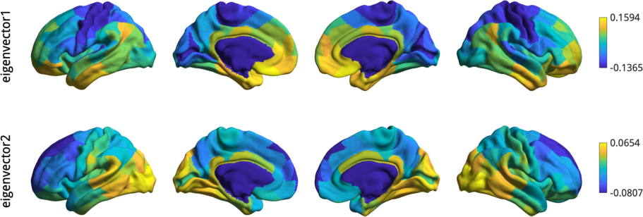
We then use this output in the fit function. This will convert the long horizontal array into a square affinity matrix, and then perform embedding.

% resolve the gradients
gm = GradientMaps('kernel','na');
gm = gm.fit(fused_matrix, 'Sparsity', 0);
h = plot_hemispheres(gm.gradients{1}(:,1:2), ...
        {surf_lh,surf_rh}, ...
         'parcellation', labeling, ...
         'labeltext',{'eigenvector1','eigenvector2'});

Note

The mpc matrix presented here match the subject cohort of (Paquola et al., 2019). Other matrices in this package match the subject groups used by (Vos de Wael et al., 2018). We make direct comparisons in our tutorial for didactic purposes only.

That concludes the second tutorial. In the third tutorial we will consider null hypothesis testing of comparisons between gradients and other markers.