Tutorial 1: Building your first gradient
In this example, we will derive a gradient and do some basic inspections to determine which gradients may be of interest and what the multidimensional organization of the gradients looks like.
We’ll first start by loading some sample data. Note that we’re using parcellated data for computational efficiency.
% First load mean connectivity matrix and Schaefer parcellation
conn_matrix = load_group_fc('schaefer',400);
labeling = load_parcellation('schaefer',400);

% The loader functions output data in a struct array for when you
% load multiple parcellations. Let's just bring them to numeric arrays.
conn_matrix = conn_matrix.schaefer_400;
labeling = labeling.schaefer_400;

% and load the conte69 hemisphere surfaces
[surf_lh, surf_rh] = load_conte69();
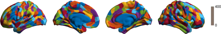
Let’s first look at the parcellation scheme we’re using.
h = plot_hemispheres(labeling, {surf_lh,surf_rh});
colormap(h.handles.figure,lines(401))
and let’s construct our gradients.
% Construct the gradients
gm = GradientMaps();
gm = gm.fit(conn_matrix);
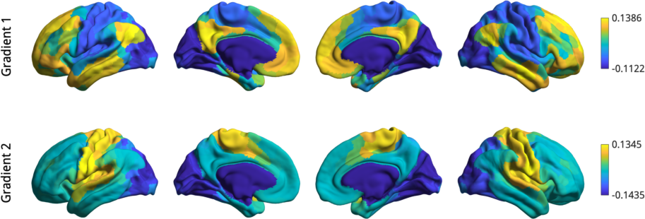
Note that the default parameters (normalized angle kernel, diffusion embedding approach, 10 components) will be reported in the console. Once you have your gradients a good first step is to simply inspect what they look like. Let’s have a look at the first two gradients.
plot_hemispheres(gm.gradients{1}(:,1:2),{surf_lh,surf_rh}, ...
             'parcellation', labeling, ...
             'labeltext',{'Gradient 1','Gradient 2'});
But which gradients should you keep for your analysis? In some cases you may have an a-priori interest in some previously defined set of gradients. When you don not have a pre-defined set, you can instead look at the lambdas (eigenvalues) of each component in a scree plot. Higher eigenvalues (or lower in laplacian eigenmapping) are more important, so one can choose a cut-off based on a scree plot.
scree_plot(gm.lambda{1});

A reasonable choice based on this scree plot would be to focus on the first two gradients as they provide a good trade-off between keeping few components whilst retaining a large amount of variance.
Inspecting gradients together can be quite informative. BrainSpace provides tools for plotting a set of gradients in 2D or 3D space, and assigning them colors based on their position. This color can then be propagated to the surface to get an idea of the multidimensional interaction between the gradients. You do this as follows:
gradient_in_euclidean(gm.gradients{1}(:,1:2));
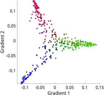
We can see that the values of each region are relatively clustered along three lines, colored here in red, green, and blue. If we want to put these colors on the cortical surface, we simply provide the same function with the surface (and parcellation if using parcellated data).
gradient_in_euclidean(gm.gradients{1}(:,1:2),{surf_lh,surf_rh},labeling);
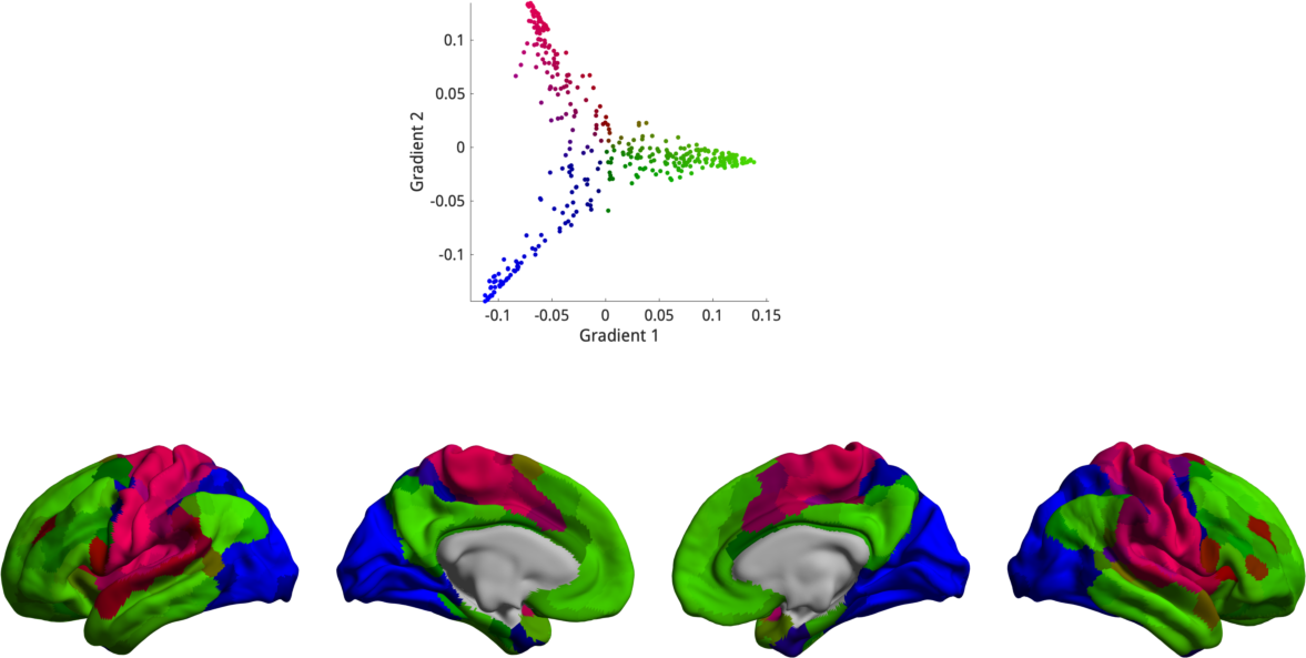
It now becomes quite evident that the three lines we see in the scatter plot correspond to the somatomotor (red), default mode (green) and visual (blue) networks.
This concludes the first tutorial. In the next tutorial we will have a look at how to customize the methods of gradient estimation, as well as gradient alignments.