Tutorial 3: Null models for gradient significance
In this tutorial we assess the significance of correlations between the first canonical gradient and data from other modalities (curvature, cortical thickness and T1w/T2w image intensity). A normal test of the significance of the correlation cannot be used, because the spatial auto-correlation in MRI data may bias the test statistic. In this tutorial we will show two approaches for null hypothesis testing: spin permutations and Moran spectral randomization.
Note
When using these approaches to compare gradients to non-gradient markers, we recommend randomizing the non-gradient markers as these randomizations need not maintain the statistical independence between gradients.
Spin Permutations
Here, we use the spin permutations approach previously proposed in (Alexander-Bloch et al., 2018), which preserves the auto-correlation of the permuted feature(s) by rotating the feature data on the spherical domain. We will start by loading the conte69 surfaces for left and right hemispheres, their corresponding spheres, midline mask, and t1w/t2w intensity as well as cortical thickness data, and a template functional gradient.
% load the conte69 hemisphere surfaces and spheres
[surf_lh, surf_rh] = load_conte69;
[sphere_lh, sphere_rh] = load_conte69('spheres');

% Load the data
[t1wt2w_lh,t1wt2w_rh] = load_marker('t1wt2w');
[thickness_lh,thickness_rh] = load_marker('thickness');

% Template functional gradient
embedding = load_gradient('fc',1);
Let’s first generate some null data using spintest.
% Let's create some rotations
n_permutations = 1000;
y_rand = spin_permutations({[t1wt2w_lh,thickness_lh],[t1wt2w_rh,thickness_rh]}, ...
                  {sphere_lh,sphere_rh}, ...
                  n_permutations,'random_state',0);

% Merge the rotated data into single vectors
t1wt2w_rotated = squeeze([y_rand{1}(:,1,:); y_rand{2}(:,1,:)]);
thickness_rotated = squeeze([y_rand{1}(:,2,:); y_rand{2}(:,2,:)]);
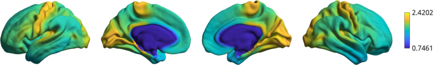
As an illustration of the rotation, let’s plot the original t1w/t2w data
% Plot original data
h1 = plot_hemispheres([t1wt2w_lh;t1wt2w_rh],{surf_lh,surf_rh});
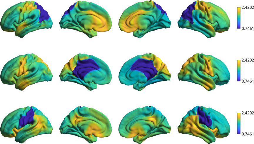
as well as a few rotated version.
% Plot a few of the rotations
h2 = plot_hemispheres(t1wt2w_rotated(:,1:3),{surf_lh,surf_rh});
Warning
Depending on the overlap of midlines (i.e. NaNs) in the original data and in the rotation, statistical comparisons between them may compare different numbers of features. This can bias your test statistics. Therefore, if a large portion of the sphere is not used, we recommend using Moran spectral randomization instead.
Now we simply compute the correlations between the first gradient and the original data, as well as all rotated data.
% Find correlation between FC-G1 with thickness and T1w/T2w
[r_original_thick, pval_thick_spin] = corr(embedding,[thickness_lh;thickness_rh], ...
                'rows','pairwise','type','spearman');
% pval_thick_spin = 0

[r_original_t1wt2w, pval_t1wt2w_spin] = corr(embedding,[t1wt2w_lh;t1wt2w_rh], ...
                'rows','pairwise','type','spearman');
% pval_t1wt2w_spin = 0

r_rand_thick = corr(embedding,thickness_rotated, ...
            'rows','pairwise','type','spearman');
r_rand_t1wt2w = corr(embedding,t1wt2w_rotated, ...
            'rows','pairwise','type','spearman');
To find a p-value, we simply compute the percentile rank of the true correlation in the distribution or random correlations. Assuming a threshold of p<0.05 for statistical significance and disregarding multiple comparison corrections, we consider the correlation to be significant if it is lower or higher than the 2.5th/97.5th percentile, respectively.
% Compute percentile rank.
 prctile_rank_thick = mean(r_original_thick > r_rand_thick);
 % prctile_rank_thick = 0.9410

 prctile_rank_t1wt2w = mean(r_original_t1wt2w > r_rand_t1wt2w);
 % prctile_rank_t1wt2w = 0

 significant_thick = prctile_rank_thick < 0.025 || prctile_rank_thick >= 0.975;
 significant_t1wt2w = prctile_rank_t1wt2w < 0.025 || prctile_rank_t1wt2w >= 0.975;
If significant is true, then we have found a statistically significant correlation. Alternatively, one could also test the one-tailed hypothesis whether the percentile rank is lower or higher than the 5th/95th percentile, respectively.
Moran Spectral Randomization
Moran Spectral Randomization (MSR) computes Moran’s I, a metric for spatial auto-correlation and generates normally distributed data with similar auto-correlation. MSR relies on a weight matrix denoting the spatial proximity of features to one another. Within neuroimaging, one straightforward example of this is inverse geodesic distance i.e. distance along the cortical surface.
In this example we will show how to use MSR to assess statistical significance between cortical markers (here curvature and cortical t1wt2w intensity) and the first functional connectivity gradient. We will start by loading the conte69 surfaces for left and right hemispheres, a left temporal lobe mask, t1w/t2w intensity as well as cortical thickness data, and a template functional gradient.
% load the conte69 hemisphere surfaces and spheres
[surf_lh, surf_rh] = load_conte69();

% Load the data
t1wt2w_lh = load_marker('t1wt2w');
curv_lh = load_marker('curvature');

% Load mask
temporal_mask_tmp = load_mask('temporal');

% There's a one vertex overlap between the HCP midline mask (i.e. nans) and
% our temporal mask.
temporal_mask_lh = temporal_mask_tmp & ~isnan(t1wt2w_lh);

% Load the embedding
embedding = load_gradient('fc',1);
embedding_lh = embedding(1:end/2);

% Keep only the temporal lobe.
embedding_tl = embedding(temporal_mask_lh);
t1wt2w_tl = t1wt2w_lh(temporal_mask_lh);
curv_tl = curv_lh(temporal_mask_lh);
We will now compute the Moran eigenvectors. This can be done either by providing a weight matrix of spatial proximity between each vertex, or by providing a cortical surface (see also: compute_mem). Here we’ll use a cortical surface.
n_ring = 1;
MEM = compute_mem(surf_lh,'n_ring',n_ring,'mask',~temporal_mask_lh);
Using the Moran eigenvectors we can now compute the randomized data. As the computationally intensive portion of MSR is mostly in compute_mem, we can push the number of permutations a bit further.
n_rand = 10000;
y_rand = moran_randomization([curv_tl,t1wt2w_tl],MEM,n_rand, ...
    'procedure','singleton','joint',true,'random_state',0);

curv_rand = squeeze(y_rand(:,1,:));
t1wt2w_rand = squeeze(y_rand(:,2,:));
Now that we have the randomized data, we can compute correlations between the gradient and the real/randomized data.
[r_original_curv,pval_curv_moran] = corr(embedding_tl,curv_tl,'type','spearman');
% pval_curv_moran = 6.6380e-05

[r_original_t1wt2w,pval_t1wt2w_moran] = corr(embedding_tl,t1wt2w_tl,'type','spearman');
% pval_t1wt2w_moran = 0

r_rand_curv = corr(embedding_tl,curv_rand,'type','spearman');
r_rand_t1wt2w = corr(embedding_tl,t1wt2w_rand,'type','spearman');
To find a p-value, we simply compute the percentile rank of the true correlation in the distribution or random correlations. Assuming a threshold of p<0.05 for statistical significance and disregarding multiple comparison corrections, we consider the correlation to be significant if it is lower or higher than the 2.5th/97.5th percentile, respectively.
prctile_rank_curv = mean(r_original_curv > r_rand_curv);
% prctile_rank_curv = 0.8249

prctile_rank_t1wt2w = mean(r_original_t1wt2w > r_rand_t1wt2w);
% prctile_rank_t1wt2w = 0

significant_curv = prctile_rank_curv < 0.025 || prctile_rank_curv >= 0.975;
significant_t1wt2w = prctile_rank_t1wt2w < 0.025 || prctile_rank_t1wt2w >= 0.975;
If significant is true, then we have found a statistically significant correlation. Alternatively, one could also test the one-tailed hypothesis whether the percentile rank is lower or higher than the 5th/95th percentile, respectively.
There are some scenarios where MSR results do not follow a normal distribution. It is relatively simple to check whether this occurs in our data by visualizing the null distributions. Check this interesting paper for more information (Burt et al.,2020).
% Compute the correlations between real and random data.
upper_triangle = triu(ones(size(curv_rand,2),'logical'),1);
r_real_rand_curv = corr(curv_tl,curv_rand);
r_real_rand_t1wt2w = corr(t1wt2w_tl,t1wt2w_rand);
r_rand_rand_curv = corr(curv_rand);
r_rand_rand_t1wt2w = corr(t1wt2w_rand);
r_rand_rand_curv = r_rand_rand_curv(upper_triangle);
r_rand_rand_t1wt2w = r_rand_rand_t1wt2w(upper_triangle);

% Plot histograms
figure('Color','w');
subplot(2,2,1);
hist(r_real_rand_curv,100);
title('Correlation curvature real and random');
subplot(2,2,2);
hist(r_real_rand_t1wt2w,100);
title('Correlation t1w/t2w real and random');
subplot(2,2,3);
hist(r_rand_rand_curv,100);
title('Correlation curvature random and random');
subplot(2,2,4);
hist(r_rand_rand_t1wt2w,100);
title('Correlation curvature random and random');
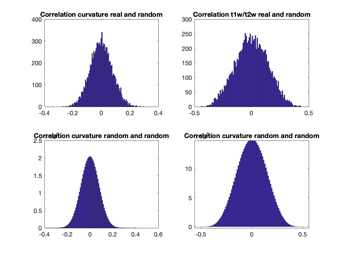
Indeed, our histograms appear to be normally distributed. This concludes the third and last tutorial. You should now be familliar with all the functionality of the BrainSpace toolbox. For more details on any specific function, please see MATLAB Package.
Variogram Matching
Here, we use the variogram matching presented in (Burt et al., 2020), which generates novel brainmaps with similar spatial autocorrelation to the input data. We will start by loading the conte69 surfaces for left and right hemispheres, a left temporal lobe mask, t1w/t2w intensity as well as cortical thickness data.
% load the conte69 hemisphere surfaces and spheres
[surf_lh, surf_rh] = load_conte69();

% Load the data
t1wt2w_lh = load_marker('t1wt2w');
curv_lh = load_marker('curvature');

% Load mask
temporal_mask_tmp = load_mask('temporal');

% There's a one vertex overlap between the HCP midline mask (i.e. nans) and
% our temporal mask.
temporal_mask_lh = temporal_mask_tmp & ~isnan(t1wt2w_lh);

% Load the embedding
embedding = load_gradient('fc',1);
embedding_lh = embedding(1:end/2);

% Keep only the temporal lobe.
t1wt2w_tl = t1wt2w_lh(temporal_mask_lh);
curv_tl = curv_lh(temporal_mask_lh);
Next, we will need a distance matrix that tells us what the spatial distance between our datapoints is. For this example, we will use geodesic distance.
G = surface_to_graph(surf_lh, 'geodesic', ~temporal_mask_lh, true);
geodesic_distance = distances(G);
Now we’ve got everything we need to generate our surrogate datasets. By default, BrainSpace will use all available data to generate surrogate maps. However, this process is extremely computationally and memory intensive. When using this method with more than a few hundred regions, we recommend subsampling the data. This can be done using the ‘ns’ and ‘knn’ name-value pairs. ‘ns’ determines how many data points to sample for the generation of the variogram; ‘knn’ determines how many neighbors to use in the smoothing step.
random_initialization = 0;
n_surrogate_datasets = 10;

% Note: num_samples must be greater than num_neighbors
num_samples = 200;
num_neighbors = 100;

obj_subsample = variogram(geodesic_distance, 'ns', num_samples, ...
    'knn', num_neighbors, 'random_state', random_initialization);
surrogates_subsample = obj_subsample.fit(t1wt2w_tl, n_surrogate_datasets);
Note
The variogram class also supports parallel processing with the ‘num_workers’ Name-Value pair. This functionality requires the Parallel Computing Toolbox.
The correlation between the real data, surrogate data, and the marker of interest can then be compared as follows. Note that, for this example, we only generated 10 surogate datasets. For any practical usage we recommend generating at least 1000.
r_real = corr(t1wt2w_tl, curv_tl);
r_surrogate = corr(surrogates_subsample, curv_tl);
prctile_rank = mean(r_real > r_surrogate);