Getting Started

Introduction to Gradients

Classically, many neuroimaging studies have attempted to parcellate the human brain into distinct areas based on anatomical or functional features. Whilst effective, the strict boundaries assumed by these methods are often unrealistic and there lacks a clear ordering between parcels. More recently, “gradient” approaches, which define the brain as a set of continuous scores along manifold axes, have gained popularity (see also References). Core to these techniques is the computation of an affinity matrix that captures inter-area similarity of a given feature followed by the application of dimensionality reduction techniques to identify a gradual ordering of the input matrix in a lower dimensional manifold space.

BrainSpace is a compact and flexible toolbox that implements a wide variety of approaches to build macroscale gradients from neuroimaging and connectome data. In this overview, we will show the the basic steps needed for the identi cation of gradients, and their visualization. The steps below will help you to get started and to build your first gradients. If you haven’t done so yet, we recommend you install the package (Installation Guide) so you can follow along with the examples.

Basic Gradient Construction

The packages comes with the conte69 surface, and several cortical features and parcellations. Let’s start by loading the conte69 surfaces:

Python

Matlab

>>> from brainspace.datasets import load_conte69

>>> # Load left and right hemispheres
>>> surf_lh, surf_rh = load_conte69()
>>> surf_lh.n_points
32492

>>> surf_rh.n_points
32492

addpath(genpath('/path/to/micasoft/BrainSpace/matlab'));

% Load left and right hemispheres
[surf_lh, surf_rh] = load_conte69();

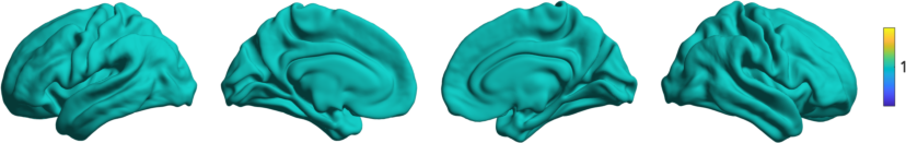
To load your own surfaces, you can use the read_surface function. BrainSpace also provides surface plotting functionality. We can plot the conte69 surfaces as follows:

Python

Matlab

>>> from brainspace.plotting import plot_hemispheres

>>> plot_hemispheres(surf_lh, surf_rh, size=(800, 200))

plot_hemispheres(ones(64984,1),{surf_lh,surf_rh});

Let’s also load the mean connectivity matrix built from a subset of the human connectome project (HCP). The package comes with several example matrices, downsampled using the Schaefer parcellations (Schaefer et al., 2017). Let’s load one of them.

Python

Matlab

>>> from brainspace.datasets import load_group_fc, load_parcellation

>>> labeling = load_parcellation('schaefer', scale=400, join=True)
>>> m = load_group_fc('schaefer', scale=400)
>>> m.shape
(400, 400)

labeling = load_parcellation('schaefer',400);
conn_matices = load_group_fc('schaefer',400);
m = conn_matices.schaefer_400;

To compute the gradients of our connectivity matrix m we create the GradientMaps object and fit the model to our data:

Python

Matlab

>>> from brainspace.gradient import GradientMaps

>>> # Build gradients using diffusion maps and normalized angle
>>> gm = GradientMaps(n_components=2, approach='dm', kernel='normalized_angle')

>>> # and fit to the data
>>> gm.fit(m)
GradientMaps(alignment=None, approach='dm', kernel='normalized_angle',
             n_components=2, random_state=None)

>>> # The gradients are in
>>> gm.gradients_.shape
(400, 2)

% Build gradients using diffusion maps and normalized angle
gm = GradientMaps('kernel','na','approach','dm','n_components',2);

% and fit to the data
gm = gm.fit(m);

Now we can visually inspect the gradients. Let’s plot the first gradient:

Python

Matlab

>>> import numpy as np
>>> from brainspace.utils.parcellation import map_to_labels

>>> # map to original size
>>> grad = map_to_labels(gm.gradients_[:, 0], labeling, mask=labeling != 0,
...                      fill=np.nan)

>>> # Plot first gradient on the cortical surface.
>>> plot_hemispheres(surf_lh, surf_rh, array_name=grad, size=(800, 200))

% Plot the first gradient on the cortical surface.
plot_hemispheres(gm.gradients{1}(:,1), {surf_lh,surf_rh}, ...
        'parcellation',labeling.schaefer_400);

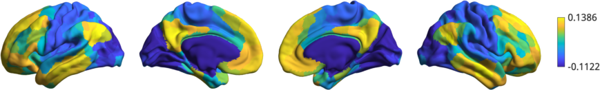
As we can see, this gradient corresponds to those observed previously in the literature i.e. running from default mode to sensory areas.

That concludes this getting started section. For more full documentation and tutorials please see MATLAB Package and/or Python Package.